Overview
Google BigQuery is a fully managed data warehouse with advanced functionality and pre-built features like machine learning, geospatial analysis, and business intelligence tooling.
BigQuery’s scalable, distributed analysis engine allows for hyper-efficient querying and data manipulation. Given its serverless architecture and self-managed implementation, little warehouse management is required.
BigQuery stores data using a columnar format, optimized for analytical queries and compatible with database transaction semantics (ACID). Additionally, BigQuery provides centralized management of all data and compute resources, secured through Google’s Identity and Access Management (IAM), which provides secure, yet flexible, security management— whether following Google’s best practices or taking a more granular approach.
 Matt Palmer
Architecture
Externalization of Dremel
Google BigQuery is the public implementation of Dremel— a distributed system developed at Google for interactively querying large datasets. BigQuery provides the core set of features available in Dremel to third-party developers through a REST API, a command line tool, and a Web UI.
Dremel, and by extension BigQuery, can scan billions of rows without an index in tens of seconds. For example, taken from Google’s whitepaper on the subject, Dremel is capable of performing a Regex match on 314 million rows of Wikipedia data to return an aggregated result in 10 seconds.
It’s important to understand the underlying technology to fully grasp the power of using Google BigQuery as a data warehouse. BigQuery’s foundation enables super high scalability and efficiency.
Columnar Storage

BigQuery is a column-based data warehouse, which powers its speed and ability to handle enormous quantities of data. In many databases, data is stored and accessed by row. While efficient for transactional databases (updating records is much quicker), analytical databases are faster when stored by column, since in many analytic queries only a few columns are read at a time— for example,
SELECT
	DATE(event_timestamp) as date,
	SUM(purchase_amount) as revenue
FROM cleaned.purchases
GROUP BY date
ORDER BY date
will return the sum of purchase amount (revenue) by date. A column-based service only needs to read...
event_timestamp & purchase_amount...while a row-based service would have to scan every row of the dataset.
Typically, organizations might store many columns in such a table, hence column-based datastores allow for efficient querying of wide tables. BigQuery is one of the first implementations of a columnar storage-based analytics system used in-conjunction with parallel processing.
Additional efficiency gains can be made by making use of BigQuery’s partitioning and clustering features, which we’ll discuss separately.
Tree Architecture
Tree architecture is a method of dispatching queries and collecting results using parallel computing. Since BigQuery is a managed, serverless service, commands are executed across tens of thousands of machines in a matter of seconds. Tree architecture allows for that functionality.

Tree architecture forms a massively parallel distributed tree for pushing down a query, then aggregating results from leaves at blistering speeds. Queries are disaggregated into bits of logic that can be dispatched across thousands of machines, then reaggregated into a result.
The combination of Tree architecture and columnar-based storage allowed Google to implement the distributed design for the technology underlying BigQuery, and powers the performance and cost advantages of the system over competitors.

BigQuery vs. MapReduce
MapReduce is a big data technology that’s existed longer than Google’s Dremel and BigQuery— it’s better known by the open source implementation Hadoop. Also a distributed computing technology, MapReduce allows for programmatic implementation of custom mapper and reducer functions. These can then run across batch processes on hundreds or thousands of servers.

Example MapReduce data flow for extracting counts from text.
BigQuery differs from MapReduce since:
- BigQuery is an interactive data analysis tool for large datasets.
- MapReduce is designed as a programming framework to batch process large datasets.
While MapReduce is efficient at batch processing large datasets for demanding data conversion or aggregation, it is not well suited for ad hoc querying due to its speed. MapReduce is much better suited for programming complex logic and processing unstructured data than BigQuery, but it is not very useful for OLAP (Online Analytical Processing) or BI (Business Intelligence).
BigQuery is designed to handle structured data using SQL. Hence, it’s more efficient at finding particular records under specified conditions, quick aggregation of statistics with dynamic conditions, and trial-and-error data analysis.

Federated Querying
While many data teams rely on an ETL pipeline (extract, transform, load) using a service like Apache Beam, Apache Spark or Zuar Runner, it is possible to implement similar functionality within Google BigQuery. Since BigQuery separates compute from storage, SQL queries may be run against CSV or JSON files stored in Google Cloud Storage. This is known as federated querying.
Federated querying can be leveraged to extract data from Google Cloud Storage, transform the data, and materialize results into a BigQuery table using SQL. Even if transformation isn’t necessary, BigQuery can directly ingest standard data formats natively. Data can then be mutated or queried directly (EL: extract load, or ELT: extract load transform).
This simplifies the complexity of data pipelines and reduces the quantity of tools necessary to accomplish some data goals. This functionality can provide cost savings, but there are limitations...
- Federated queries aren't supported in all regions
- There are quota limits on cross-region federated querying
- Calculating the bytes billed before actually executing the federated queries isn't possible
- A federated query can have at most 10 unique connections
- With federated querying in general, not all schemas are supported
- A robust ETL/ELT tool can provide a wider scope of capabilities
Related Article:
Team Zuar

BigQuery Features
BI Engine
BigQuery BI Engine is an in-memory analysis service that provides extremely fast (subsecond) query response times with high concurrency. It leverages a simplified architecture by performing in-place analysis through BigQuery, which eliminates the need for overly complex transformation pipelines. BI Engine integrates with both Google BI tools (Data Studio and Looker) as well as other popular choices for visualizing query results.
BigQuery ML
BigQuery ML allows for the creation and execution of machine learning models using standard SQL. This decreases development speed and democratizes machine learning— only SQL knowledge is necessary and data is directly accessible from BigQuery.
Historically, ML has required extensive programming knowledge of machine learning frameworks, which has restricted development to a select few. BigQuery ML makes machine learning more accessible to data analysts through existing skills, without the need to import data from multiple sources.
Connected Sheets
BigQuery has native support for exporting data to Google Sheets. This unlocks additional data manipulation and visualization functionality, but also provides an ideal access to data for financial analysts, stakeholders, and others who are used to analyzing data in a spreadsheet.
Since Google manages both services, setup is relatively simple. Connected Sheets further democratizes data and provides an important linkage between two powerful methods of analysis: the data warehouse and the spreadsheet.
An ELT tool like Runner can also bring in data from Google Sheets, while providing you with a more robust selection of tools.

Functionality
BigQuery Table Types
BigQuery supports the following table types:
- Managed Tables: Tables backed by native BigQuery Storage.
- External Tables: Tables supported by storage outside BigQuery that enables live queries against data in other systems.
- Standard Views: Virtual tables defined by a SQL query. The results for these tables are generated at runtime.
- Materialized Views: Precomputed views that periodically refresh results and persist within BigQuery.
Read more about various BigQuery table types and their use cases here.

Partitioning & Clustering
Overview
Partitioning and clustering are common methods to optimize data reads and writes. Using partitions and clusters, architects may minimize the amount of data scanned, reducing costs and improving performance.
Partitioning
Like many other data warehouses, BigQuery supports table partitioning on both date and integer fields. Date partitioning is an incredibly useful tactic for analytical databases, as it lets you scan limited columns over constrained date ranges— queries are then cost efficient and fast! In our earlier example, adding a date constraint limits the scan to the specified data partitions:
SELECT
	DATE(event_timestamp) as date,
	SUM(purchase_amount) as revenue
FROM cleaned.purchases
WHERE DATE(event_timestamp) BETWEEN CURRENT_DATE() - 60 AND CURRENT_DATE()
GROUP BY date
ORDER BY date
When used in combination with a columnar datastore, only two rows are scanned across only the desired date range—maximum query efficiency is achieved!
Clustering
Clustering is another way of organizing data—in a clustered table, data is stored by row according to similar values in the clustered columns. In BigQuery, up to 4 columns may be clustered when tables are created. It’s best to cluster tables by commonly filtered or grouped columns.
In our earlier example, we might cluster the purchases table by source if we frequently analyze data on that variable:
SELECT
	DATE(event_timestamp) as date,
	SUM(purchase_amount) as revenue
FROM cleaned.purchases
WHERE
	DATE(event_timestamp) BETWEEN CURRENT_DATE() - 60 AND CURRENT_DATE()
	AND source = ‘web’
GROUP BY date
ORDER BY date
Efficiency would then be optimized for the query above, where we’re filtering on source=’web’, since data is partitioned by date and ordered by source in the BigQuery table.

Geospatial Data
BigQuery is unique in its ability to transform and manipulate geospatial data. It uses a GEOGRAPHY data type to represent a geometry value or collection. A table with a geometry column and additional attributes can be used to represent spatial features, with the entire table representing a spatial feature collection.
A host of geospatial data functions are supported in standard SQL that allows for analysis of geographical data, construction and manipulation of GEOGRAPHY data types, and determination of spatial relationships between geographical features.
These functions are particularly helpful for analyzing mobile devices, location sensors, social media data, or satellite imagery, which can then be analyzed in graphs, maps, descriptive statistics, and cartograms.
For businesses with a large dependence on map data, polylines, or locations, BigQuery’s geography support can provide a large lift by making analysis simple, cost-effective, and accessible in pure SQL.

BigQuery UDFs
Main modern data warehouses support user-defined functions (UDFs) to organize frequently-used logic, however BigQuery is unique in that it supports both SQL and JavaScript code in UDFs. A BigQuery UDF takes columns as input, performs actions, and returns the result as a value.
UDFs may be defined as either persistent or temporary. Persistent UDFs may be reused across multiple queries, while temporary UDFs exist only in the scope of a single query. To create a BigQuery UDF, use the CREATE FUNCTION statement. An example of a SQL UDF is:
CREATE TEMP FUNCTION AddFourAndDivide(x INT64, y INT64)
  RETURNS FLOAT64
  AS ((x + 4) / y);

SELECT val, AddFourAndDivide(val, 2)
  FROM UNNEST([2,3,5,8]) AS val;
Temporary/persistent UDFs are created by including or removing the TEMP parameter. Defining JavaScript UDFs is similar:
CREATE TEMP FUNCTION multiplyInputs(x FLOAT64, y FLOAT64)
RETURNS FLOAT64
LANGUAGE js AS r"""
  return x*y;
""";

WITH numbers AS
  (SELECT 1 AS x, 5 as y
  UNION ALL
  SELECT 2 AS x, 10 as y
  UNION ALL
  SELECT 3 as x, 15 as y)
SELECT x, y, multiplyInputs(x, y) as product
FROM numbers;
See the BigQuery docs for more info.

Arrays
BigQuery is unique in its use of arrays— a BigQuery array is an ordered list containing values of the same data type. Arrays are useful wherever there’s a need for ordering, storing repeated values in a single row, or performance improvements. Storing data as arrays can reduce storage overhead and potentially speed-up queries that do not require repeated fields.
Arrays are also useful for generating data. BigQuery has several functions that allow for date and integer generation, like GENERATE_DATE_ARRAY(). In some SQL languages, generating a list of values can be a surprisingly complex task. In BigQuery, it’s rather simple. The following snippet generates a row per date for each day in 2022:
WITH year AS (
 SELECT
  GENERATE_DATE_ARRAY('2022-01-01', 2022-12-31', INTERVAL 1 DAY) AS day
)
SELECT day
FROM year, UNNEST(day) AS day
Arrays can also be manipulated (concatenated, mutated, casted) using other BigQuery array functions. For a complete list, see the BigQuery docs.

Information Schema
The BigQuery Information Schema is a series of views that provide various table metadata. Using the Information Schema, you can quickly query resource usage, pricing, views, sessions, and other table info. For example, querying the INFORMATION_SCHEMA.JOBS_BY_PROJECT table, one could aggregate cost by user email.
The following views are available in BigQuery:

Table Sampling
Table sampling is a helpful feature that allows for querying random subsets of data from large tables. Rather than performing a full table scan, it’s possible to get a subset of data, which lowers query cost and is often faster for ad-hoc analysis.
To use table sampling, append a TABLESAMPLE clause to a select statement. For example...
SELECT * FROM dataset.my_table TABLESAMPLE SYSTEM (10 PERCENT)...will select a random sample equivalent to 10 percent of the original data source. This differs from LIMIT in that TABLESAMPLE is truly random. Also, BigQuery does not cache the results of table sample queries, so the query may return different results each time! Table sampling may be used with other selection conditions, like where clauses, and joins.
This feature works by randomly selecting a percentage of data blocks (which underlie all BigQuery tables) and reading all of their rows. Typically, blocks are about 1GB in size. For tables consisting of only one block, BigQuery randomly selects rows.
Since partitioned and clustered tables produce blocks where all rows have a certain partition key or clustering attribute, sample sets from those tables may be more biased than non-partitioned, non-clustered tables. For truly random, individual-row sampling, use a WHERE rand() < K clause. The downside is that such a clause results in a full table scan and often higher costs.
Some limitations of table sampling include:
- A sampled table can only appear once in a query statement. This restriction includes tables that are referenced inside view definitions.
- Data cannot be sampled from views.
- Subqueries and table-valued function calls cannot be sampled.
- Sampling inside an IN subquery is not supported.
For more on table sampling, see the BigQuery docs.

BigQuery Security
One of the biggest advantages to a fully managed serverless product is the included, prebuilt security infrastructure. In Google Cloud Platform (GCP), data is fully encrypted, as is the API-serving infrastructure. Google’s Identity and Access Management (IAM) powers Google Cloud Platform and BigQuery. To access those resources, users and apps must be authenticated, authorized, and permissioned using IAM.
BigQuery IAM
GCP IAM works by defining and controlling three things: identity, role, and resource:
- Identity: who has access. This can be an end-user specified through email or an application, identified by a service account. Service accounts can be created to have a subset of permissions of the creator. They’re typically used for application access to Google Cloud Platform.
- Role: The role determines what access is allowed for the identity in question. A role consists of a set of permissions. BigQuery allows both predefined and custom role-sets. Predefined roles are composed of frequently required combinations of permissions. For example, the dataViewer role provides the ability to get metadata and table data, but not the ability to create or delete resources.
- Resource: Access to resources is managed individually— after assigning an identity and role, users must be granted the right to interact with specific datasets and tables.
These properties can be administered via the BigQuery web UI, the REST API, or the BQ command-line tool. Admins can create Google groups with commonly defined roles to simplify the process of administering a large organization.
Google’s security and provisioning features allow for granular control over data storage and access. Given increasing legal complexity around data governance, the robust security feature set is an essential part of the platform and adds a considerable amount of value to the solution.
According to Jeffrey Breen, Chief Product Officer of the cybersecurity company Protegrity,

BigQuery Pricing
Pricing Overview
BigQuery pricing has two main components: analysis and storage pricing. Analysis pricing is the cost to process queries, UDFs, scripts, and other data access statements, while storage pricing is the cost to store data loaded into BigQuery. Pricing accurate as of July 15, 2022.
Analysis Pricing
For analysis pricing, BigQuery offers two pricing models:
- On Demand: for on-demand pricing, BigQuery charges $5.00 per terabyte (TB) of data scanned. The first TB per month is free.
- Flat Rate: customers can either subscribe to annual or monthly flat-rate commitments. For annual agreements, the monthly analytics cost is $1,700 for 100 slots. Slots are BigQuery’s units for measuring query processing capacity.
The right pricing model will depend on the customer’s use case, but the on-demand rate tends to favor newer customers, while flat-rate pricing is typically advantageous for power users or those with large enterprise-level data needs.
Storage Pricing
BigQuery charges for two types of storage:
- Active storage: includes any table or partition that has been modified in the last 90 days.
- Long-term storage: includes any table or partition that has not been modified for 90 consecutive days.
The pricing for active storage is $0.20 per GB scanned. Long-term storage is offered at $0.10 per GB. For both types of storage, the first 10 GB per month is free. Storage pricing is prorated per MB scanned.
Data storage has become incredibly cheap over the last few decades. Nonetheless, for customers with large quantities of data, reserving large datastores for long-term storage can help to mitigate overhead.
Pricing is subject to change and differs by action, so be sure to read the BigQuery docs for up-to-date information.

Expert Help
For those looking for a fully-managed, serverless data warehouse, Google BigQuery could be a great option. But what is the next step? Data warehousing is only a piece of a larger data strategy- how can that data be extracted and analyzed?
That is where an ETL/ELT solution such as Runner comes in. Runner is an automated data pipeline solution by Zuar that takes data from a multitude of sources (data warehouses, ERP, CRM, etc.), stages it for analysis, and brings it into an analytics platform such as Tableau.
Learn more about how Runner integrates with databases, or take the next step and schedule a data assessment with Zuar!
FAQ
When should I use BigQuery?
Google BigQuery is used as a Cloud Data Warehouse— for storing processed analytical data in schemas and tables to be consumed by analysts, stakeholders, and data teams. Given the columnar-based storage, partitioning, and clustering functionality, BigQuery is ideal for quickly storing and re-accessing data to be disseminated within an organization (or for personal projects).
Is Google BigQuery a database?
No, Google BigQuery is a managed cloud data warehouse, which has more functionality than a traditional database. While BigQuery has database features, it is also more complex and fully-functioned. Databases exist within Google BigQuery, but BigQuery itself is not a database.
What is BigQuery vs SQL?
Google BigQuery is a managed cloud data warehouse, whereas SQL (Structured Query Language) is a language for interfacing with databases. BigQuery does have its own SQL variant, BigQuery SQL, with advanced functionality and modern features.
Is BigQuery SQL or NoSQL?
BigQuery is a SQL data warehouse. Google BigQuery is a Cloud columnar oriented database built on Google’s Dremel technology. Data is stored by column in tables and organized into schemas, where it may be queried and mutated using BigQuery SQL.
What is the difference between Bigtable and BigQuery?
Google Bigtable is a NoSQL wide-column database. It's optimized for low latency, large numbers of reads and writes, and maintaining performance at scale. Bigtable use cases are of a certain scale or throughput with strict latency requirements, such as IoT, AdTech, FinTech, and so on. Google BigQuery is an enterprise data warehouse for large amounts of relational structured data. It is optimized for large-scale, ad-hoc SQL-based analysis and reporting, which makes it best suited for gaining organizational insights. You can even use BigQuery to analyze data from Cloud Bigtable.
What is a dataset in BigQuery?
A BigQuery dataset refers to a table stored on the service. BigQuery is a column-based database system, so tables stored on BigQuery are scanned by column and partition. Furthermore, BigQuery is a SQL Cloud Data Warehouse, meaning that tables (datasets) are accessed through BigQuery SQL.
How is data stored in BigQuery?
BigQuery is a column-based data warehouse, which powers its speed and ability to handle enormous quantities of data. In many databases, data is stored and accessed by row. While efficient for transactional databases (updating records is much quicker), analytical databases are faster when stored by column, since in many analytic queries only a few columns are read at a time. BigQuery is one of the first implementations of a columnar storage-based analytics system used in-conjunction with parallel processing. BigQuery also supports partitioning and clustering, two techniques for organizing stored data and optimizing query costs.
Is BigQuery free?
No, while Google BigQuery does have a free trial and free usage tier, BigQuery is a paid service, like most cloud data warehouses. For nearly all functionality, the cost of BigQuery will scale with usage, meaning that the solution will be very inexpensive for smaller teams. Often, BigQuery costs can be mitigated through price-optimization and adhering to best practices. See the BigQuery Pricing Page for more information.